SBC and calibration

library(bayesim)

Introduction

Simulation-based calibration (SBC) checks Bayesian inference against data generated from the model (Talts et al., 2018):

If we draw a parameter theta from the model prior, simulate data y from the likelihood given theta, and then fit the model to y, the resulting rank of theta among independent posterior draws should be uniform across repeated simulations.

Equivalently, the posterior rank of the true theta among the posterior draws should be uniformly distributed on {0, 1, ..., S}. Departures can indicate errors in inference or in the simulation setup.

The coverage guarantee averages over parameters drawn from the prior and data drawn from the likelihood. It does not guarantee nominal coverage at each fixed parameter value. Rank checks can detect errors that a check of one credible interval misses, but passing SBC does not establish that an inference algorithm is correct.

This vignette uses LinearRegressionFitter() for exact conjugate Normal-Inverse-Gamma Bayesian linear regression without Stan. For Stan/brms models, swap the fitter for BrmsFitter() or CmdStanFitter() and use prior_predictive_generator() / ifs_generator(); the SBC workflow below is identical. One caveat: prior_predictive_generator() draws theta from the model prior (valid SBC by construction when the fitting prior matches), but ifs_generator() draws theta from a preconditioning posterior, so its ranks are only uniform if the fitting prior is set to match that preconditioning distribution. An unmatched fitting prior can produce nonuniform ranks without a sampler error (see ?ifs_generator).

Running SBC

The SBC recipe needs three ingredients:

A data generator that draws theta from the model prior and simulates y ~ p(y | theta).
A fitter whose calibration we want to check.
The rank metric (rank_metric()), which counts how many posterior draws fall below the true theta, giving one rank per task per parameter.

Below, the generator draws (Intercept, slope, sigma) from exactly the same Normal-Inverse-Gamma prior passed to LinearRegressionFitter(), then simulates Gaussian linear data. In an NIG prior the coefficient distribution is conditional on the residual variance: beta | sigma^2 ~ Normal(0, sigma^2 Lambda^-1). Matching that conditional prior is essential; a prior mismatch is itself a valid SBC failure mode. Because the fitter is the exact conjugate updater for this same prior, SBC should pass by construction.

sbc_generator <- function(data_spec, task_ctx) {
  n <- data_spec$n
  # Exact NIG prior used by the fitter below:
  # sigma^2 ~ Inv-Gamma(2, 1)
  # beta | sigma^2 ~ Normal(0, sigma^2 / 0.25)
  sigma     <- sqrt(1 / stats::rgamma(1, shape = 2, rate = 1))
  intercept <- stats::rnorm(1, mean = 0, sd = sigma / sqrt(0.25))
  slope     <- stats::rnorm(1, mean = 0, sd = sigma / sqrt(0.25))
  # Simulate y from the likelihood given theta.
  x <- stats::rnorm(n)
  y <- intercept + slope * x + stats::rnorm(n, sd = sigma)
  list(
    train = data.frame(y = y, x = x),
    test = NULL,
    response = "y",
    true_params = c(Intercept = intercept, x = slope, sigma = sigma),
    vars_of_interest = c("Intercept", "x", "sigma")
  )
}

The data generator uses the current RNG state. bayesim restores a per-task L’Ecuyer stream before each call, so do not call set.seed() inside (see vignette("reproducibility")).

Now configure and run the study. We use 150 replicates and 1000 posterior draws per fit, with rank_metric(thin = "auto") so the rank counts are adjusted for autocorrelation in the draws (here the NIG draws are i.i.d., so no thinning is needed, but the option is there for MCMC-based fitters).

config <- simulation_config(
  data_grid = data.frame(n = 40L),
  fit_grid = data.frame(model = "lm"),
  data_generator = sbc_generator,
  fitter = LinearRegressionFitter(
    n_draws = 1000L,
    prior_mean = 0,
    prior_precision = 0.25,
    a0 = 2,
    b0 = 1
  ),
  metrics = list(
    rank_metric(thin = "auto"),
    posterior_summary_metric()
  ),
  n_replicates = 150L,
  seed = 7L
)

result <- run_simulation(config, progress = FALSE)
#> 150 tasks = 1 data x 1 fit x 150 reps
#> ℹ Starting simulation with 150 tasks
#> 
#> ✔ Simulation complete: 150/150 tasks succeeded in 1.6s

Each task records one rank per parameter (here Intercept, x, sigma), plus the posterior summaries needed for the coverage check below.

Checking rank uniformity

sbc_ranks() collects the per-task ranks into a long tibble; plot_rank_ecdf() plots the empirical CDF of the normalized ranks against the uniform CDF (the diagonal), with the simultaneous uniformity band of Säilynoja, Bürkner, and Vehtari (2022).

ranks <- sbc_ranks(result)
head(ranks)
#>                      task_id     param rank n_draws n_ranks data_n fit_model
#> Intercept.1 d001_f001_r00001 Intercept  920    1000    1001     40        lm
#> Intercept.2 d001_f001_r00002 Intercept  148    1000    1001     40        lm
#> Intercept.3 d001_f001_r00003 Intercept  680    1000    1001     40        lm
#> Intercept.4 d001_f001_r00004 Intercept  254    1000    1001     40        lm
#> Intercept.5 d001_f001_r00005 Intercept  826    1000    1001     40        lm
#> Intercept.6 d001_f001_r00006 Intercept  902    1000    1001     40        lm

plot_rank_ecdf(ranks, alpha = 0.95)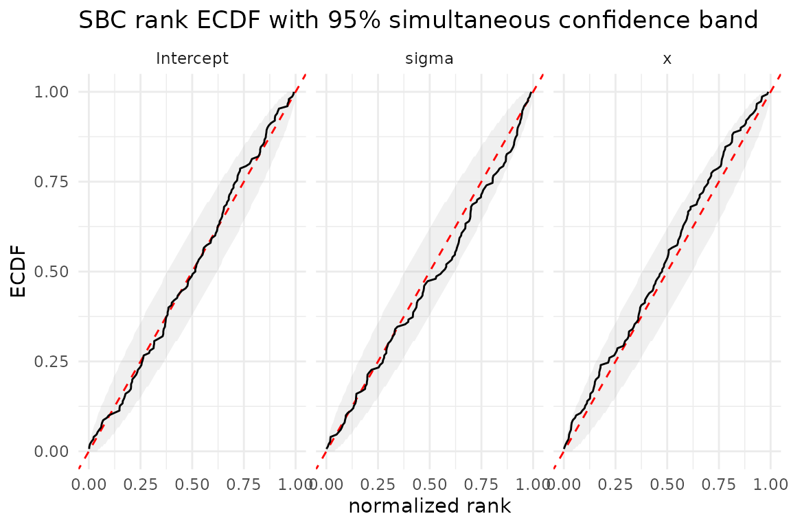

The red diagonal is the uniform CDF. The grey ribbon is a 95% simultaneous band: for independent uniform ranks on a common support, the whole ECDF stays inside it in about 95% of repetitions. This level applies to each panel separately. A crossing can occur by chance even with exact inference.

If condition cells share truth draws, their ranks are dependent. Pooling them can make the band too narrow. Use by to separate the conditions, for example plot_rank_ecdf(result, by = c("data_n", "fit_model")) when those columns identify the cells. The band does not correct for dependence from shared draws (#59). It is also approximate when ranks within a panel have different supports.

Interpreting departures

The shape can suggest a cause, but does not identify it uniquely:

ECDF relative to the diagonal	Possible explanation
Above on the left, below on the right	Posterior uncertainty is too small.
Below on the left, above on the right	Posterior uncertainty is too large.
Mostly above	Posterior estimates tend to exceed the truth.
Mostly below	Posterior estimates tend to fall below the truth.

Check the generator, model, and sampler diagnostics before attributing a departure to the inference method. More replicates improve the ability to detect small departures.

Coverage as a complementary check

SBC checks the whole posterior at once. A complementary, more familiar check is interval coverage: does the nominal 95% credible interval contain the truth about 95% of the time? plot_coverage() shows this per estimand with MCSE error bars; performance_measures() reports the same quantity in a table. Because SBC draws a new truth from the prior for every replicate, this is a varying-truth study. Accordingly, the table labels error summaries as mean_error, error_sd, and error_mse; it does not label them as the fixed-truth Morris measures bias, emp_se, or mse.

plot_coverage(result)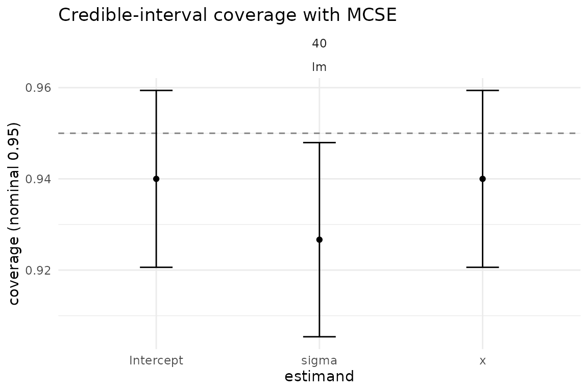

pm <- performance_measures(result, estimand = "x")
pm
#> # A tibble: 6 × 8
#>   data_n fit_model estimand measure       value     mcse n_sim truth_mode
#>    <int> <chr>     <chr>    <chr>         <dbl>    <dbl> <int> <chr>     
#> 1     40 lm        x        mean_error   0.0209  0.0122    150 varying   
#> 2     40 lm        x        error_sd     0.150   0.00869   150 varying   
#> 3     40 lm        x        error_mse    0.0228  0.00396   150 varying   
#> 4     40 lm        x        model_se     0.140   0.00441   150 varying   
#> 5     40 lm        x        coverage     0.94    0.0194    150 varying   
#> 6     40 lm        x        n_sim      150      NA         150 varying

The coverage row reports the empirical coverage of the 95% posterior interval for the x coefficient, with its Monte Carlo standard error. For the conjugate fitter this should sit close to the nominal 0.95 (within a couple of MCSEs). The truth_mode column is "varying". Here mean_error is the average replicate-level difference estimate - truth, and its MCSE is computed from those replicate-level errors; error_sd describes the spread of that error distribution. These are useful calibration summaries, but they are not the empirical sampling SE or bias of an estimator at one fixed truth.

Coverage checks one interval level. Rank uniformity checks calibration over a range of posterior quantiles for the quantities supplied to rank_metric(). Neither check proves that every aspect of the joint posterior is correct. Use a fixed-truth generator when you want the estimator-performance measures bias, emp_se, and mse.

Introduction

Running SBC

Checking rank uniformity

Interpreting departures

Coverage as a complementary check

Further reading