Design of simulation studies

library(bayesim)

Introduction

A simulation study is an experiment whose subjects are datasets simulated from a known data-generating process (DGP), and whose measurements are the performance of one or more estimators applied to those datasets. Because the truth is known, simulation is the gold standard for evaluating statistical methods — but only when the study itself is well-designed and honestly reported.

This vignette follows the framework of Morris, White & Crowther (2019, Statistics in Medicine), which structures a simulation study around four questions:

1. What are the estimands — the quantities we want the method to recover?
2. What are the data-generating mechanisms — the DGPs that produce the simulated datasets, and how do they expose the estimands?
3. What are the performance measures — bias, variance/SE, MSE, coverage, etc. — used to judge the method, and what is their Monte Carlo standard error (MCSE)?
4. How many replicates are needed to estimate those performance measures to acceptable precision, and across which varying conditions?

bayesim provides typed primitives for each of these. This vignette runs end-to-end with LinearRegressionFitter() (exact conjugate Bayesian linear regression, no Stan) so every chunk is executable.

Estimands and data-generating mechanisms

The estimand is the target of inference — the parameter whose value the method is supposed to recover. In a simulation, the estimand is known because we set it. bayesim records it automatically: any name in a generator’s true_params vector becomes a truth__<param> column in the per-task summary (see vignette("getting-started")), and that column is what the analysis layer pairs against the per-task posterior estimate.

The data-generating mechanism is the function that turns a parameter setting into a dataset. bayesim generators have the signature (data_spec, task_ctx) -> data_bundle and must consume the ambient RNG state (the engine restores a per-task L’Ecuyer stream before each call; do not re-seed inside). The factory constructors fixed_truth_generator(), prior_predictive_generator(), and ifs_generator() cover common patterns; for everything else, write an inline generator like the one below.

# A linear-regression DGP. The estimands (Intercept, slope x, sigma) are
# recorded as true_params; bayesim surfaces them as truth__* columns.
linear_dgp <- function(data_spec, task_ctx) {
  n <- data_spec$n
  beta <- data_spec$beta
  x <- stats::rnorm(n)
  y <- 1 + beta * x + stats::rnorm(n)
  list(
    train = data.frame(y = y, x = x),
    test = NULL,
    response = "y",
    true_params = c(Intercept = 1, x = beta, sigma = 1),
    vars_of_interest = c("Intercept", "x", "sigma")
  )
}

The data_grid is the table of data_spec rows swept over. Each row is one data-generating condition; each condition is replicated n_replicates times.

Performance measures

The performance measures of Morris et al. (2019) characterise an estimator across replicate datasets:

• bias — does the estimator hit the truth on average?
• empirical SE (emp_se) — how variable is the estimator across datasets?
• MSE — mean squared error, the combined bias-plus-variance.
• coverage — does the nominal interval contain the truth at the nominal rate?
• model SE (model_se) — the average uncertainty the method itself reports (compare to the empirical SE to check the method’s uncertainty calibration).

Each of these is a Monte Carlo estimate from n replicates, so each carries an MCSE — the simulation’s own standard error. Reporting a performance estimate without its MCSE is like reporting a sample mean without a standard error: the reader cannot tell signal from noise. bayesim computes every MCSE for you.

Run a small study and call performance_measures():

config <- simulation_config(
  data_grid = data.frame(n = 100L, beta = 0.5),
  fit_grid = data.frame(model = "lm"),
  data_generator = linear_dgp,
  fitter = LinearRegressionFitter(n_draws = 400L),
  metrics = list(posterior_summary_metric()),
  n_replicates = 80L,
  seed = 11L
)

result <- run_simulation(config, progress = FALSE)
#> 80 tasks = 1 data x 1 fit x 80 reps
#> ℹ Starting simulation with 80 tasks
#> 
#> ✔ Simulation complete: 80/80 tasks succeeded in 0.6s

pm <- performance_measures(result, estimand = "x")
pm
#> # A tibble: 6 × 9
#>   data_n data_beta fit_model estimand measure    value     mcse n_sim truth_mode
#>    <int>     <dbl> <chr>     <chr>    <chr>      <dbl>    <dbl> <int> <chr>     
#> 1    100       0.5 lm        x        bias     -0.0211  1.22e-2    80 fixed     
#> 2    100       0.5 lm        x        emp_se    0.110   8.71e-3    80 fixed     
#> 3    100       0.5 lm        x        mse       0.0123  2.11e-3    80 fixed     
#> 4    100       0.5 lm        x        model_se  0.0979  9.96e-4    80 fixed     
#> 5    100       0.5 lm        x        coverage  0.938   2.71e-2    80 fixed     
#> 6    100       0.5 lm        x        n_sim    80      NA          80 fixed

The tidy tibble has one row per estimand x measure, with the value and its mcse. For the conjugate fitter on this DGP we expect: bias near zero, emp_se and model_se close to each other (the posterior correctly reports its own uncertainty), and coverage near the nominal 0.95.

The MCSE formulas follow Morris et al. / rsimsum: bias MCSE = sd / sqrt(n); emp_se MCSE = sd / sqrt(2(n-1)); MSE MCSE via the delta method on the squared errors; coverage MCSE = sqrt(p(1-p) / n); model_se MCSE = sd(posterior_sd) / sqrt(n). These are exactly the formulas inverted by n_replicates_for_target() below.

How many replicates?

The MCSE shrinks as 1/sqrt(n), so the number of replicates is a precision budget. n_replicates_for_target() inverts the MCSE formulas to tell you how many replicates you need to hit a target MCSE before you run the study — a power calculation for simulation.

For coverage, the MCSE is sqrt(p(1-p) / n), maximised at p = 0.5 (the conservative default). Inverting gives n = p(1-p) / MCSE^2.

# Target: coverage MCSE of 0.03 at the conservative p = 0.5.
n_replicates_for_target(target_mcse = 0.03, metric_type = "coverage")
#> [1] 278

So 278 replicates (ceiling) are needed to estimate a coverage rate to within +/- 0.03 (one MCSE) at the worst-case variance. If the coverage is expected near the nominal 0.95, supply p = 0.95 for a tighter, smaller estimate:

n_replicates_for_target(target_mcse = 0.03, metric_type = "coverage", p = 0.95)
#> [1] 53

For a continuous measure (bias, model SE), the MCSE is sd / sqrt(n), so you must supply an assumed standard deviation for the per-replicate point estimate (e.g. a guess at the empirical SE of the estimator, perhaps from a pilot run):

# Target bias MCSE of 0.05, assuming the point estimate has sd ~ 0.5.
n_replicates_for_target(
  target_mcse = 0.05, metric_type = "continuous", assumed_sd = 0.5
)
#> [1] 100

Use these numbers to size the study up front: a coverage claim with 50 replicates and MCSE 0.07 is barely more precise than a coin flip, while 1,000+ replicates give MCSEs near 0.015 — the difference between a defensible simulation and an anecdotal one.

Varying conditions

A simulation study that varies nothing proves nothing about the range of behaviour a method exhibits. The Morris et al. framework emphasises sweeping over the factors that plausibly change performance: sample size, effect size, noise level, model mis-specification, etc. In bayesim, varying conditions are just additional rows in the data_grid (or columns swept within it); the analysis layer’s by argument then groups the performance measures by condition.

Below we vary sample size and effect size together:

design_config <- simulation_config(
  data_grid = data.frame(
    n = c(60, 60, 120, 120),
    beta = c(0.5, 1.0, 0.5, 1.0)
  ),
  fit_grid = data.frame(model = "lm"),
  data_generator = linear_dgp,
  fitter = LinearRegressionFitter(n_draws = 400L),
  metrics = list(posterior_summary_metric()),
  n_replicates = 60L,
  seed = 23L
)

design_result <- run_simulation(design_config, progress = FALSE)
#> 240 tasks = 4 data x 1 fit x 60 reps
#> ℹ Starting simulation with 240 tasks
#> 
#> ✔ Simulation complete: 240/240 tasks succeeded in 1s

Group the performance measures by both conditions with the by argument. The data_grid columns surface in the summary with a data_ prefix, so we group by data_n and data_beta:

pm_design <- performance_measures(
  design_result, estimand = "x", by = c("data_n", "data_beta")
)
pm_design
#> # A tibble: 24 × 8
#>    data_n data_beta estimand measure     value     mcse n_sim truth_mode
#>     <dbl>     <dbl> <chr>    <chr>       <dbl>    <dbl> <int> <chr>     
#>  1     60       0.5 x        bias     -0.00245  0.0158     60 fixed     
#>  2     60       0.5 x        emp_se    0.122    0.0112     60 fixed     
#>  3     60       0.5 x        mse       0.0147   0.00279    60 fixed     
#>  4     60       0.5 x        model_se  0.130    0.00205    60 fixed     
#>  5     60       0.5 x        coverage  0.95     0.0281     60 fixed     
#>  6     60       0.5 x        n_sim    60       NA          60 fixed     
#>  7     60       1   x        bias     -0.0164   0.0177     60 fixed     
#>  8     60       1   x        emp_se    0.137    0.0126     60 fixed     
#>  9     60       1   x        mse       0.0187   0.00264    60 fixed     
#> 10     60       1   x        model_se  0.126    0.00230    60 fixed     
#> # ℹ 14 more rows

Read each row as one condition cell. As n grows, the empirical SE and MSE should shrink (more data, tighter inference); as beta grows the signal strengthens. Coverage should stay near 0.95 throughout for the conjugate fitter. The MCSE column tells you how much trust to put in each cell at 60 replicates — a reminder that small condition x condition grids with few replicates produce noisy performance estimates.

Plotting coverage across conditions gives the visual version of the coverage rows. plot_coverage() plots each condition x estimand cell as a point with MCSE error bars against the nominal rate:

plot_coverage(design_result, by = c("data_n", "data_beta"))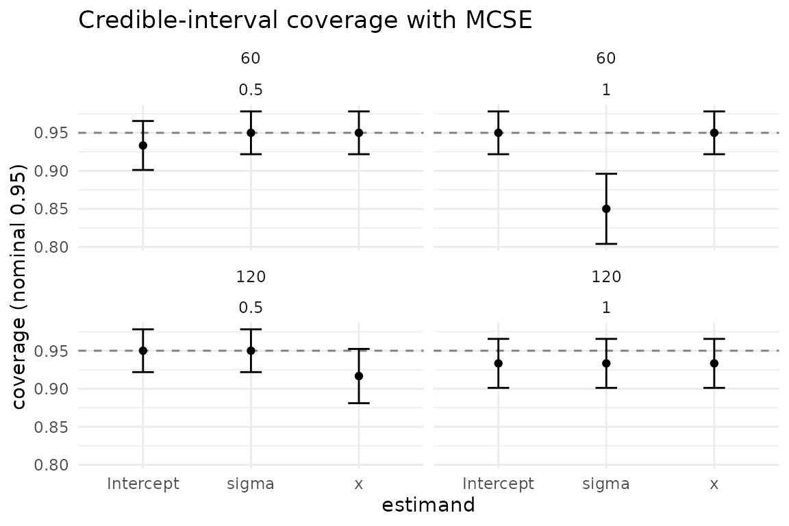

For a fuller picture, plot_recovery() shows per-task posterior-mean estimates against the truth, faceted by a condition column — a direct visual check that the estimator recovers the estimand across the design:

plot_recovery(design_result, estimand = "x", by = "data_n")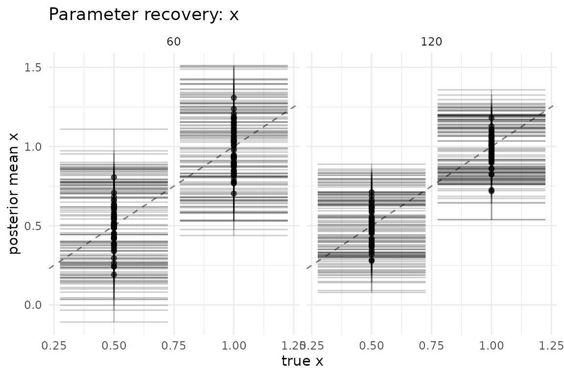

The parameter argument is named estimand, the same term performance_measures() uses (var = remains accepted as a compatibility alias).

Summary

The Morris et al. (2019) framework, in bayesim, maps to a small set of typed primitives:

• Estimands are recorded by generators as true_params and surfaced as truth__* columns.
• DGPs are generators (fixed_truth_generator(), prior_predictive_generator(), ifs_generator(), or an inline function).
• Performance measures with MCSEs come from performance_measures().
• Replicate sizing comes from n_replicates_for_target().
• Varying conditions are rows/columns of the data_grid, grouped in the analysis layer via by.

For the calibration-specific counterpart to performance coverage — checking the whole posterior for self-consistency rather than a single interval — see vignette("sbc-and-calibration").

Reference

Morris, White & Crowther (2019), Using simulation studies to evaluate statistical methods, Statistics in Medicine 38(11): 2074-2102.