Creating Efficacy Tables

Introduction

Create efficacy tables for clinical study reports: time-to-event analysis, response rates, subgroup analyses, and change from baseline endpoints.

Setup and Data Preparation

library(pharmhand)
library(dplyr)
library(tidyr)
library(ggplot2)
library(survival)

# Set flextable defaults for readable tables in light/dark mode
flextable::set_flextable_defaults(
  font.color = "#000000",
  background.color = "#FFFFFF"
)

Use pharmaverseadam for example data:

library(pharmaverseadam)

# Load example datasets
adsl <- pharmaverseadam::adsl         # Subject-level data
advs <- pharmaverseadam::advs         # Vital signs data
adlb <- pharmaverseadam::adlb         # Laboratory data
adtte <- pharmaverseadam::adtte_onco  # Time-to-event data (oncology)
adrs <- pharmaverseadam::adrs_onco    # Response data (oncology)

# Note: adtte_onco and adrs_onco use ARM as treatment variable (not TRT01P)

Time-to-Event Analysis

create_tte_summary_table() provides survival analysis with Kaplan-Meier estimates, hazard ratios, and landmark analyses.

Basic TTE

# Create TTE summary table
# Note: adtte_onco uses ARM for treatment groups
tte_table <- create_tte_summary_table(
  data = adtte,
  time_var = "AVAL",
  event_var = "CNSR",
  trt_var = "ARM",  # Use ARM instead of TRT01P for oncology data
  title = "Overall Survival Summary"
)

# Display the table
tte_table@flextable

Overall Survival Summary
Statistic	Placebo	Xanomeline High Dose	Xanomeline Low Dose
N	174	169	169
Events n (%)	5 (2.9)	3 (1.8)	2 (1.2)
Median (95% CI)	NE	NE	NE
HR (95% CI)	Reference	0.84 (0.20, 3.53)	0.56 (0.11, 2.92)
p-value	-	0.809	0.492
FAS Population
Time unit: months
HR reference group: Placebo
NE = Not Estimable

TTE with Landmarks

# TTE table with landmark survival estimates
tte_landmark <- create_tte_summary_table(
  data = adtte,
  time_var = "AVAL",
  event_var = "CNSR",
  trt_var = "ARM",
  landmarks = c(12, 24),  # 12 and 24 month survival rates
  time_unit = "months",
  title = "Progression-Free Survival with Landmark Analysis"
)

# Display the table
tte_landmark@flextable

Progression-Free Survival with Landmark Analysis
Statistic	Placebo	Xanomeline High Dose	Xanomeline Low Dose
N	174	169	169
Events n (%)	5 (2.9)	3 (1.8)	2 (1.2)
Median (95% CI)	NE	NE	NE
12-months Rate (95% CI)	97.8 (94.8, 100.0)	97.8 (94.8, 100.0)	97.8 (94.8, 100.0)
24-months Rate (95% CI)	97.8 (94.8, 100.0)	97.8 (94.8, 100.0)	97.8 (94.8, 100.0)
HR (95% CI)	Reference	0.84 (0.20, 3.53)	0.56 (0.11, 2.92)
p-value	-	0.809	0.492
FAS Population
Time unit: months
HR reference group: Placebo
NE = Not Estimable

Kaplan-Meier Plots

# Basic KM plot
km_plot <- create_km_plot(
  data = adtte,
  time_var = "AVAL",
  event_var = "CNSR",
  trt_var = "ARM",
  title = "Overall Survival Kaplan-Meier Plot",
  show_median = TRUE,
  show_ci = TRUE,
  xlab = "Days"
)
km_plot@plot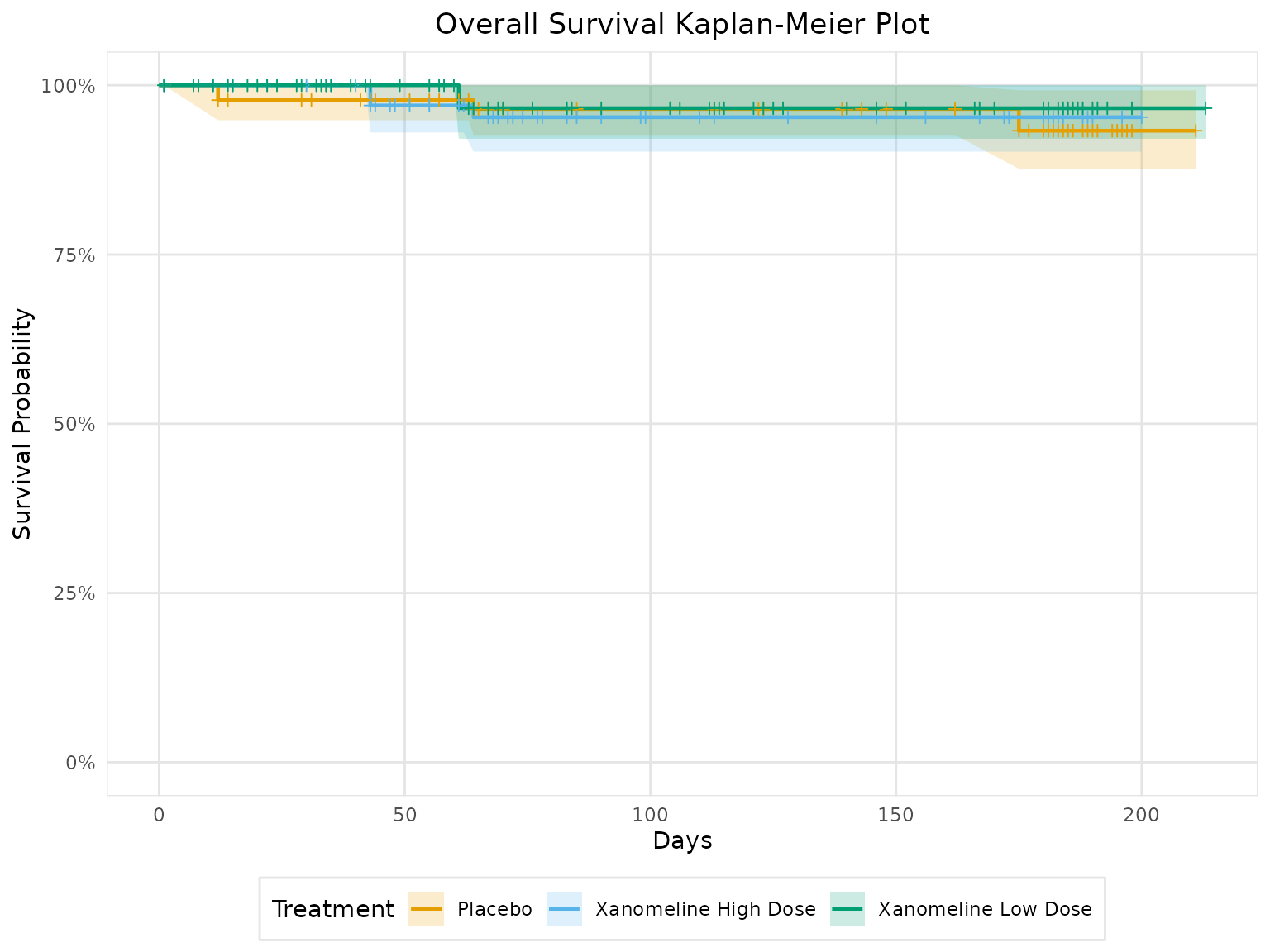

# Advanced KM plot with risk table
km_plot_advanced <- create_km_plot(
  data = adtte,
  time_var = "AVAL",
  event_var = "CNSR",
  trt_var = "ARM",
  title = "Survival Analysis with Risk Table",
  show_median = TRUE,
  show_ci = TRUE,
  xlab = "Days",
  risk_table = TRUE,
  landmarks = c(12, 24)
)
km_plot_advanced@plot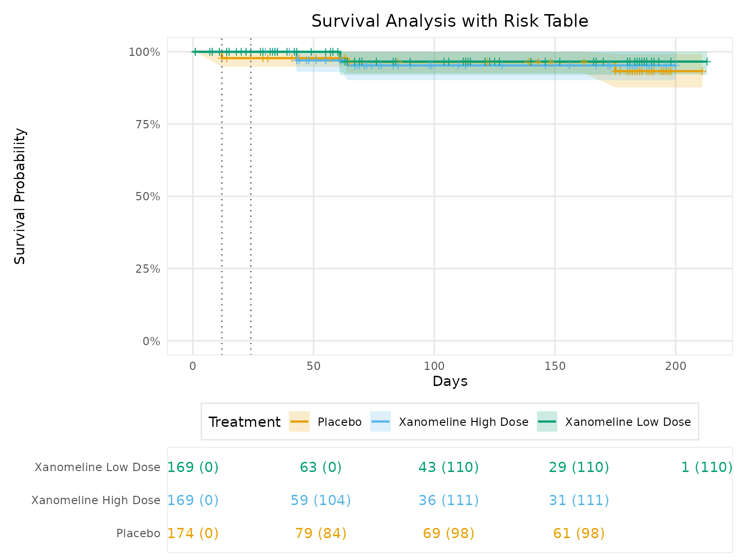

Proportional Hazards Diagnostics

Use Schoenfeld residual tests, log-log plots, and automatic warnings to validate Cox model assumptions across time-to-event analyses.

# Schoenfeld residual test with optional diagnostic plot
ph_results <- test_ph_assumption(
  data = adtte,
  time_var = "AVAL",
  event_var = "CNSR",
  trt_var = "ARM",
  plot = TRUE
)
ph_results$results
ph_results$plot@plot

# Log-log survival plot for visual PH assessment
loglog_plot <- create_loglog_plot(
  data = adtte,
  time_var = "AVAL",
  event_var = "CNSR",
  trt_var = "ARM",
  title = "Log-log Survival Plot"
)
loglog_plot@plot

# create_tte_summary_table() checks PH by default (check_ph = TRUE)

Responder Analysis

create_responder_table() provides response summaries with multiple comparison options.

Basic Response

# Create response rate table for tumor response
# Note: adrs_onco uses ARM for treatment groups
response_table <- create_responder_table(
  data = adrs,
  response_var = "AVALC",
  response_values = c("CR", "PR"),  # CR + PR = Overall Response Rate
  trt_var = "ARM",
  title = "Best Overall Response Rate"
)

# Display the table
response_table@flextable

Best Overall Response Rate
Treatment	n/N	Rate (%)	95% CI	OR (95% CI)	p-value
Placebo	8/1042	0.8	(0.4, 1.5)	Reference	-
Xanomeline High Dose	3/1016	0.3	(0.1, 0.9)	0.38 (0.10, 1.45)	0.157
Xanomeline Low Dose	4/1012	0.4	(0.2, 1.0)	0.51 (0.15, 1.71)	0.277
Screen Failure	0/624	0.0	(0.0, 0.6)	0.00 (0.00, Inf)	0.989
Response defined as: CR, PR
95% CI calculated using wilson method
OR compared to Placebo

Response with Risk Ratio

# Response table using risk ratio instead of odds ratio
response_rr <- create_responder_table(
  data = adrs,
  response_var = "AVALC",
  response_values = c("CR", "PR"),
  trt_var = "ARM",
  comparison_type = "RR",  # Risk Ratio
  ci_method = "wilson",    # Wilson confidence interval
  title = "Response Rate Summary (Risk Ratio)"
)

# Display the table
response_rr@flextable

Response Rate Summary (Risk Ratio)
Treatment	n/N	Rate (%)	95% CI	RR (95% CI)	p-value
Placebo	8/1042	0.8	(0.4, 1.5)	Reference	-
Xanomeline High Dose	3/1016	0.3	(0.1, 0.9)	0.38 (0.10, 1.45)	0.226
Xanomeline Low Dose	4/1012	0.4	(0.2, 1.0)	0.51 (0.16, 1.70)	0.387
Screen Failure	0/624	0.0	(0.0, 0.6)	0.10 (0.01, 1.70)	0.029
Response defined as: CR, PR
95% CI calculated using wilson method
RR compared to Placebo

Response with Risk Difference

# Response table with risk difference
response_rd <- create_responder_table(
  data = adrs,
  response_var = "AVALC",
  response_values = c("CR", "PR"),
  trt_var = "ARM",
  comparison_type = "RD",  # Risk Difference
  title = "Response Rate Difference"
)

# Display the table
response_rd@flextable

Response Rate Difference
Treatment	n/N	Rate (%)	95% CI	RD (95% CI)	p-value
Placebo	8/1042	0.8	(0.4, 1.5)	Reference	-
Xanomeline High Dose	3/1016	0.3	(0.1, 0.9)	-0.5 (-1.1, 0.2)	0.139
Xanomeline Low Dose	4/1012	0.4	(0.2, 1.0)	-0.4 (-1.0, 0.3)	0.266
Screen Failure	0/624	0.0	(0.0, 0.6)	-0.8 (-1.3, -0.2)	0.005
Response defined as: CR, PR
95% CI calculated using wilson method
RD compared to Placebo

Subgroup Analysis

Subgroup analyses show treatment effects across patient populations.

Subgroup Table

# Create subgroup analysis table
subgroup_table <- create_subgroup_table(
  data = adtte,
  subgroups = list(
    SEX = "Sex"
  ),
  endpoint_type = "tte",  # Time-to-event endpoint
  trt_var = "ARM",
  title = "Subgroup Analysis - Overall Survival"
)

# Display the table
subgroup_table@flextable

Subgroup Analysis - Overall Survival
Subgroup	Category	n (Placebo)	n (Xanomeline High Dose)	HR (95% CI)	Interaction p
Overall		174	338	0.84 (0.20, 3.53)
Sex	F	107	181	1.49 (0.21, 10.61)	0.249
Sex	M	67	157	0.47 (0.05, 4.62)
HR = Hazard Ratio
Reference group: Placebo
Interaction p-value from likelihood ratio test
NE = Not Estimable

Forest Plot

# Create forest plot for subgroup analysis
forest_plot <- create_forest_plot(
  data = adtte,
  subgroups = list(
    SEX = "Sex"
  ),
  endpoint_type = "tte",
  trt_var = "ARM",
  title = "Treatment Effect by Subgroup",
  show_interaction = TRUE
)
forest_plot@plot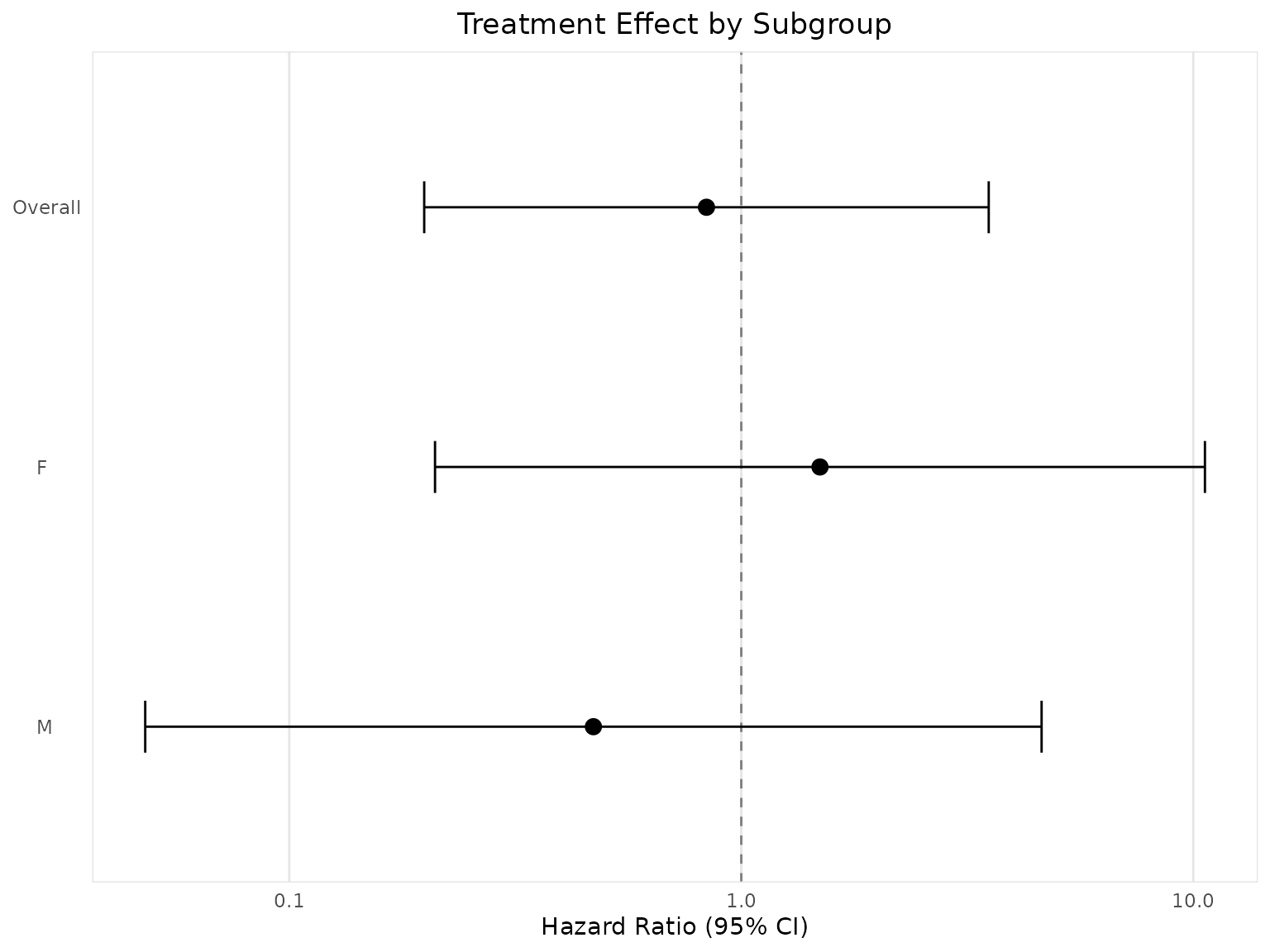

Binary Endpoint

# Subgroup analysis for binary endpoint
subgroup_binary <- create_subgroup_table(
  data = adrs,
  subgroups = list(
    SEX = "Sex"
  ),
  endpoint_type = "binary",  # Binary endpoint
  response_var = "AVALC",
  response_values = c("CR", "PR"),
  trt_var = "ARM",
  title = "Response Rate by Subgroup"
)

# Display the table
subgroup_binary@flextable

Response Rate by Subgroup
Subgroup	Category	n (Placebo)	n (Screen Failure)	OR (95% CI)	Interaction p
Overall		1042	2652	0.00 (0.00, Inf)
Sex	F	639	1517	0.00 (0.00, Inf)	0.009
Sex	M	403	1135	0.00 (0.00, Inf)
OR = Odds Ratio
Reference group: Placebo
Interaction p-value from likelihood ratio test
NE = Not Estimable

Change from Baseline Analysis

create_cfb_summary_table() analyzes change from baseline values for continuous endpoints.

Vital Signs

# Create change from baseline table for vital signs
cfb_table <- create_cfb_summary_table(
  data = advs,
  params = c("SYSBP", "DIABP", "PULSE"),
  visit = "End of Treatment",
  title = "Change from Baseline in Vital Signs"
)

# Display the table
cfb_table@flextable

Change from Baseline in Vital Signs
Parameter	Placebo n	Xanomeline High Dose n	Xanomeline Low Dose n	Placebo Mean (SD)	Xanomeline High Dose Mean (SD)	Xanomeline Low Dose Mean (SD)
Diastolic Blood Pressure (mmHg)	222	168	177	-3 (9)	-2.74 (11.34)	0.11 (10.12)
Pulse Rate (beats/min)	222	168	177	1.63 (10.7)	1.2 (8.93)	4.29 (10.39)
Systolic Blood Pressure (mmHg)	222	168	177	-3.56 (17.82)	-6.74 (14.96)	-3.7 (14.06)
FAS Population
Mean (SD) presented for change from baseline

Custom Parameters

# Change from baseline for specific parameters
cfb_custom <- create_cfb_summary_table(
  data = advs,
  params = c("SYSBP"),  # Only systolic blood pressure
  visit = "Week 8",
  title = "Systolic Blood Pressure Change from Baseline at Week 8"
)

# Display the table
cfb_custom@flextable

Systolic Blood Pressure Change from Baseline at Week 8
Parameter	Placebo n	Xanomeline High Dose n	Xanomeline Low Dose n	Placebo Mean (SD)	Xanomeline High Dose Mean (SD)	Xanomeline Low Dose Mean (SD)
Systolic Blood Pressure (mmHg)	219	168	180	0.05 (15.09)	-3.64 (15.93)	-1.17 (17.25)
FAS Population
Mean (SD) presented for change from baseline

Primary Endpoint Tables

create_primary_endpoint_table() creates summary tables for primary and secondary endpoints.

Primary Endpoint

# Create primary endpoint summary table
primary_table <- create_primary_endpoint_table(
  data = advs,
  paramcd = "SYSBP",
  visit = "End of Treatment",
  title = "Primary Endpoint Summary: Systolic Blood Pressure"
)

# Display the table
primary_table@flextable

Primary Endpoint Summary: Systolic Blood Pressure
Statistic	Placebo	Xanomeline High Dose	Xanomeline Low Dose
n	222	168	177
Mean (SD)	132.7 (15.44)	132.3 (15.62)	133 (17.08)
Median	131	131	130
Min, Max	78, 172	100, 177	92, 178
FAS Population
Parameter: SYSBP at End of Treatment

Secondary Endpoint

# Secondary endpoint analysis
secondary_table <- create_primary_endpoint_table(
  data = advs,
  paramcd = "DIABP",
  visit = "Week 8",
  title = "Secondary Endpoint: Diastolic Blood Pressure at Week 8"
)

# Display the table
secondary_table@flextable

Secondary Endpoint: Diastolic Blood Pressure at Week 8
Statistic	Placebo	Xanomeline High Dose	Xanomeline Low Dose
n	292	224	240
Mean (SD)	75.2 (9.12)	77.4 (9.07)	75.4 (10.59)
Median	76	78.3	74
Min, Max	49, 101	54, 98	52, 100
FAS Population
Parameter: DIABP at Week 8

Laboratory Analysis

Analyze laboratory parameters with shift tables and summary statistics.

Lab Summary

Click to expand: Laboratory Parameters Summary

# Create laboratory parameters summary
lab_summary <- create_lab_summary_table(
  data = adlb,
  params = c("HGB", "WBC", "PLAT", "ALT", "AST"),
  visit = "Week 24",
  title = "Laboratory Parameters Summary at Week 24"
)

# Display the table
lab_summary@flextable

Laboratory Parameters Summary at Week 24
Parameter	Placebo n	Xanomeline High Dose n	Xanomeline Low Dose n	Placebo Mean (SD)	Xanomeline High Dose Mean (SD)	Xanomeline Low Dose Mean (SD)
Alanine Aminotransferase (U/L)	57	30	26	17.86 (15.61)	20.97 (8.7)	18.19 (9.17)
Aspartate Aminotransferase (U/L)	57	30	26	25.19 (21.02)	24.43 (7.29)	22.42 (10.78)
Hemoglobin (mmol/L)	58	30	25	8.32 (0.82)	8.88 (0.85)	8.38 (0.69)
Platelet (10^9/L)	57	29	24	238.75 (51.89)	238.34 (67.53)	249.71 (63.44)
Leukocytes (10^9/L)	58	30	25	6.67 (1.77)	6.74 (1.8)	6.29 (1.84)
Safety Population
Mean (SD) presented

Lab Shift

Click to expand: Lab Shift Table

# Create laboratory shift table for liver function test
shift_table <- create_lab_shift_table(
  data = adlb,
  paramcd = "ALT",
  visit = "Week 24",
  title = "ALT Shift from Baseline to Week 24"
)

# Display the table
shift_table@flextable

ALT Shift from Baseline to Week 24
Planned Treatment for Period 01	Baseline Reference Range Indicator	NORMAL	HIGH	LOW
Placebo	NORMAL	51	2	1
Xanomeline High Dose	NORMAL	28	0	0
Xanomeline Low Dose	NORMAL	24	2	0
Xanomeline High Dose	HIGH	2	0	0
Placebo	HIGH	3	0	0
Safety Population
Shift from baseline normal range indicator

Vital Signs by Visit

create_vs_by_visit_table() tracks vital signs across study visits.

Click to expand: Vital Signs by Visit Table

# Vital signs by visit table
vs_visit_table <- create_vs_by_visit_table(
  data = advs,
  paramcd = "SYSBP",
  visits = c("Baseline", "Week 2", "Week 4", "Week 8", "End of Treatment"),
  title = "Systolic Blood Pressure by Study Visit"
)

# Display the table
vs_visit_table@flextable

Systolic Blood Pressure by Study Visit
Visit	Placebo	Xanomeline High Dose	Xanomeline Low Dose
Baseline	340 / 136.8 (17.57)	336 / 138.8 (18.52)	336 / 136.9 (17.27)
Week 2	336 / 133.8 (17.54)	325 / 132.3 (16.37)	335 / 135.2 (17.42)
Week 4	328 / 133.9 (17.37)	292 / 132.2 (16.14)	288 / 135.4 (17.79)
Week 8	292 / 136.3 (17.02)	224 / 135.1 (15.54)	240 / 134.9 (17.84)
End of Treatment	222 / 132.7 (15.44)	168 / 132.3 (15.62)	177 / 133 (17.08)
FAS Population
Format: n / Mean (SD)

Customization

Functions include options for confidence intervals, formatting, and custom parameters.

Formatting

# Custom formatting options
custom_table <- create_tte_summary_table(
  data = adtte,
  time_var = "AVAL",
  event_var = "CNSR",
  trt_var = "ARM",
  conf_level = 0.95,
  time_unit = "months",
  title = "Custom Formatted TTE Table",
  autofit = TRUE  # Auto-adjust column widths
)

# Display the table
custom_table@flextable

Custom Formatted TTE Table
Statistic	Placebo	Xanomeline High Dose	Xanomeline Low Dose
N	174	169	169
Events n (%)	5 (2.9)	3 (1.8)	2 (1.2)
Median (95% CI)	NE	NE	NE
HR (95% CI)	Reference	0.84 (0.20, 3.53)	0.56 (0.11, 2.92)
p-value	-	0.809	0.492
FAS Population
Time unit: months
HR reference group: Placebo
NE = Not Estimable

CI Methods

# Different CI methods for response rates
wilson_table <- create_responder_table(
  data = adrs,
  response_var = "AVALC",
  response_values = c("CR", "PR"),
  trt_var = "ARM",
  ci_method = "wilson",      # Wilson score interval (recommended)
  title = "Response Rate - Wilson CI"
)

exact_table <- create_responder_table(
  data = adrs,
  response_var = "AVALC",
  response_values = c("CR", "PR"),
  trt_var = "ARM",
  ci_method = "exact",       # Clopper-Pearson exact
  title = "Response Rate - Exact CI"
)

# Display the tables
wilson_table@flextable

Response Rate - Wilson CI
Treatment	n/N	Rate (%)	95% CI	OR (95% CI)	p-value
Placebo	8/1042	0.8	(0.4, 1.5)	Reference	-
Xanomeline High Dose	3/1016	0.3	(0.1, 0.9)	0.38 (0.10, 1.45)	0.157
Xanomeline Low Dose	4/1012	0.4	(0.2, 1.0)	0.51 (0.15, 1.71)	0.277
Screen Failure	0/624	0.0	(0.0, 0.6)	0.00 (0.00, Inf)	0.989
Response defined as: CR, PR
95% CI calculated using wilson method
OR compared to Placebo

exact_table@flextable

Response Rate - Exact CI
Treatment	n/N	Rate (%)	95% CI	OR (95% CI)	p-value
Placebo	8/1042	0.8	(0.3, 1.5)	Reference	-
Xanomeline High Dose	3/1016	0.3	(0.1, 0.9)	0.38 (0.10, 1.45)	0.157
Xanomeline Low Dose	4/1012	0.4	(0.1, 1.0)	0.51 (0.15, 1.71)	0.277
Screen Failure	0/624	0.0	(0.0, 0.6)	0.00 (0.00, Inf)	0.989
Response defined as: CR, PR
95% CI calculated using exact method
OR compared to Placebo

Complete Report

Combine multiple analyses into a report:

generate_efficacy_report <- function(output_path = "Efficacy_Report.docx") {

  # Section 1: Primary Endpoint Summary
  primary_content <- create_primary_endpoint_table(
    data = advs,
    paramcd = "SYSBP",
    visit = "End of Treatment",
    title = "Table 3.1: Primary Endpoint Summary (Systolic BP)"
  )

  # Section 2: Change from Baseline
  cfb_content <- create_cfb_summary_table(
    data = advs,
    params = c("SYSBP", "DIABP", "PULSE"),
    visit = "End of Treatment",
    title = "Table 3.2: Change from Baseline Summary"
  )

  # Section 3: Vital Signs by Visit
  vs_content <- create_vs_by_visit_table(
    data = advs,
    paramcd = "SYSBP",
    title = "Table 3.3: Vital Signs by Visit"
  )

  # Section 4: Laboratory Parameters
  lab_content <- create_lab_summary_table(
    data = adlb,
    title = "Table 3.4: Laboratory Parameters Summary"
  )

  # Section 5: Laboratory Shift Table
  shift_content <- create_lab_shift_table(
    data = adlb,
    paramcd = "ALT",
    title = "Table 3.5: ALT Shift from Baseline"
  )

  # Section 6: Subgroup Analysis
  subgroup_content <- create_subgroup_analysis_table(
    adsl = adsl,
    data = advs,
    title = "Table 3.6: Subgroup Analysis by Age Group"
  )

  # Create report sections
  sections <- list(
    ReportSection(
      title = "Primary Endpoint Analysis",
      section_type = "efficacy",
      content = list(primary_content)
    ),
    ReportSection(
      title = "Change from Baseline Analysis",
      section_type = "efficacy",
      content = list(cfb_content)
    ),
    ReportSection(
      title = "Vital Signs by Study Visit",
      section_type = "efficacy",
      content = list(vs_content)
    ),
    ReportSection(
      title = "Laboratory Parameters",
      section_type = "efficacy",
      content = list(lab_content)
    ),
    ReportSection(
      title = "Laboratory Shift Analysis",
      section_type = "efficacy",
      content = list(shift_content)
    ),
    ReportSection(
      title = "Subgroup Analyses",
      section_type = "efficacy",
      content = list(subgroup_content)
    )
  )

  # Create and save report
  report <- ClinicalReport(
    study_id = "CDISCPILOT01",
    study_title = "CDISC Pilot Study - Efficacy Report",
    sections = sections,
    metadata = list(
      generated_at = Sys.time(),
      package_version = as.character(packageVersion("pharmhand")),
      data_source = "pharmaverseadam",
      report_type = "efficacy"
    )
  )

  # Generate Word document
  generate_word(report, path = output_path)

  cat("Efficacy report generated:", output_path, "\n")
  invisible(report)
}

# Generate the report
generate_efficacy_report()