Getting Started with bayesgrove • bayesgrove

Fit a normal model to positive, skewed data, inspect its predictive checks, then record a review and try a lognormal model. This tutorial requires cmdstanr and CmdStan. The displayed results come from a recorded run; your sampler output may differ. See Concepts for terminology.

Create a project and fit a model

An initialized project is a directory with a .bayesgrove/ folder containing the graph, cache, and decision log. bg_use_cmdstanr() registers the Stan-backed node kinds, and bg_use_default_workflow() opts into the built-in review pack (register the backend first, so the pack sees the real node kinds rather than its generic placeholders).

library(bayesgrove)

handle <- bg_init(
  path = file.path(tempdir(), "bg-getting-started"),
  project_name = "Getting Started"
)
bg_use_cmdstanr(handle)
bg_use_default_workflow(handle)

The data are 50 skewed, strictly positive measurements. Start by fitting a normal model.

set.seed(31)
y <- round(rlnorm(50, meanlog = 0, sdlog = 0.8), 3)

bg_fit_stan() creates a data node, attaches the data, and creates and runs a fit node that uses it. The example Stan programs are included in the package.

normal_program <- system.file(
  "stan/normal_iid.stan",
  package = "bayesgrove",
  mustWork = TRUE
)

n_fit <- bg_fit_stan(
  handle,
  stan_file = normal_program,
  data = list(N = length(y), y = y),
  label = "Normal model",
  seed = 21,
  chains = 4
)

#> Starting run "run_dfbdc04b" with 1 node to execute.
#> Running node "node_66f87a33"...
#> Running node "node_7bd2286f"...
#> <bg_run_handle> run_dfbdc04b
#> • Status: succeeded
#> • Executed Nodes: 2

The fit has no divergences and good R-hats. bg_status() shows the project state, and bg_next_actions() asks the workflow pack whether any evidence needs review:

bg_status(handle)

#> $workflow_state
#> [1] "idle"
#>
#> $runnable_nodes
#> [1] 0
#>
#> $blocked_nodes
#> [1] 0
#>
#> $pending_gates
#> [1] 0
#>
#> $active_jobs
#> [1] 0
#>
#> $last_run_id
#> [1] "run_dfbdc04b"
#>
#> $health
#> [1] "ok"
#>
#> $messages
#> character(0)

guide <- bg_next_actions(handle)
guide$obligations

#> named list()

There are no obligations: the only summary is the fit’s HMC diagnostic, which reports no problems. The pack requests no further review of that summary.

Check the model’s predictions

Sampler diagnostics assess computation, not model fit. The built-in ppc node kind computes posterior-predictive p-values for a set of test statistics and stores plot-ready draws. It takes two inputs: the fit (for the yrep draws) and the data node (for the observed y). The fit’s data node is simply the fit node’s input, so we can read it off the graph:

graph <- bg_read_graph(handle)
n_data <- Filter(
  function(edge) identical(edge$to, n_fit),
  graph$edges
)[[1]]$from

n_ppc <- bg_add_node(
  handle,
  kind = "ppc",
  label = "PPC: normal model",
  inputs = c(n_fit, n_data),
  params = list(stats = c("mean", "sd", "min", "max"))
)
run <- bg_run(handle, targets = n_ppc)

#> Starting run "run_631ca2d5" with 1 node to execute.
#> Running node "node_7ea22ed9"...

The p-values compare each statistic of the observed data against its posterior-predictive distribution. Values near 0 or 1 flag features that the model reproduces poorly:

ppc_summary <- bg_read_summaries(handle, include_stale = FALSE)
ppc_summary <- Filter(
  function(s) identical(s$summary_kind, "posterior_predictive_check"),
  ppc_summary
)[[1]]
ppc_summary$severity
ppc_summary$metrics

#> [1] "warning"
#> $max
#> [1] 2e-04
#>
#> $mean
#> [1] 0.5098
#>
#> $min
#> [1] 2e-04
#>
#> $sd
#> [1] 0.5025

The model predicts negative values absent from the data (min) and fails to reproduce the largest observations (max). The mean and sd checks do not flag these problems. Posterior-predictive p-values are conservative; an unremarkable value is weak evidence of fit. Inspect the predictive plot:

bg_plot(handle, n_ppc)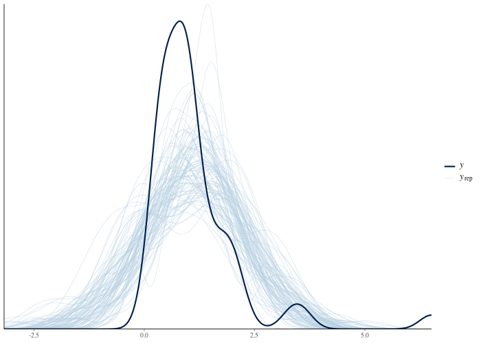

Posterior predictive density overlay for the normal model

Record a review

The summary has warning severity because of the extreme p-values. The default pack raises a blocking review_computation_validity obligation at project scope. Optional packs use more specific obligation kinds:

guide <- bg_next_actions(handle)
vapply(guide$obligations, `[[`, character(1), "kind")
vapply(guide$actions, `[[`, character(1), "kind")

#>                  obl_a969dc96
#> "review_computation_validity"
#>        act_16593cd9        act_ed08cddc
#>   "record_decision" "branch_and_modify"

An obligation identifies work needed to address the evidence and suggests actions to resolve it. Blocking obligations create execution holds. Pass these holds to the planner to prevent downstream nodes from running until the review is recorded.

held_plan <- bg_plan(handle, external_holds = guide$metadata$external_holds)
held_plan$external_blocked

#> list()

The list is empty because the failing check has no downstream nodes yet. A dependent node would be held until the obligation is resolved.

To resolve the obligation we record a decision. A decision is a permanent log entry: the prompt, the choice, the rationale, and the ids of the evidence it covers. The suggested record_decision action carries the right metadata in its payload, so we do not have to assemble it by hand:

review <- Filter(
  function(a) identical(a$kind, "record_decision"),
  guide$actions
)[[1]]

bg_record_decision(
  handle,
  scope = "project",
  prompt = "Does the normal model reproduce the data?",
  choice = "reject_normal_model",
  rationale = paste(
    "The observed minimum is far outside the posterior predictive",
    "distribution: the data are strictly positive and right-skewed,",
    "and a normal model cannot express that. Refit on the log scale."
  ),
  kind = review$payload$decision_type,
  metadata = review$payload[c("node_ids", "summary_ids")]
)

bg_next_actions(handle)$obligations

#> <bg_decision_record> dec_632c0a7b
#> • Prompt: Does the normal model reproduce the data?
#> • Choice: reject_normal_model
#> • Rationale: The observed minimum is far outside the posterior predictive
#>   distribution: the data are strictly positive and right-skewed, and a normal
#>   model cannot express that. Refit on the log scale.
#> named list()

The recorded review resolves the obligation. The summary and decision remain available so a reviewer can trace the rejection to its evidence.

Fit a lognormal model on a branch

Try the lognormal model on a branch to keep the rejected fit and its criticism in the record. bg_branch() copies the fit node into a new branch; bg_update_node() merges params, so only the Stan program changes. The default pack requires an inferential goal for each active branch. The goal records what the branch is intended to estimate.

branch <- bg_branch(handle, n_fit, label = "Lognormal model")

bg_set_goal(
  project = handle,
  branch_id = branch$branch_id,
  kind = "observable_prediction",
  label = "Positive-valued predictions",
  rationale = "The rejected normal fit motivates a lognormal likelihood."
)

lognormal_program <- system.file(
  "stan/lognormal_iid.stan",
  package = "bayesgrove",
  mustWork = TRUE
)

bg_update_node(
  handle,
  branch$root_node_id,
  params = list(stan_file = lognormal_program)
)
run2 <- bg_run(handle, targets = branch$root_node_id)

#> <bg_decision_record> dec_ca79d9cb
#> • Prompt: Set inferential goal
#> • Choice: Positive-valued predictions
#> • Rationale: The rejected normal fit motivates a lognormal likelihood.
#> [1] "node_4610511f"
#> Starting run "run_f3475fdc" with 1 node to execute.
#> Running node "node_4610511f"...

A second ppc node checks the lognormal model’s predictions:

n_ppc2 <- bg_add_node(
  handle,
  kind = "ppc",
  label = "PPC: lognormal model",
  inputs = c(branch$root_node_id, n_data),
  params = list(stats = c("mean", "sd", "min", "max"))
)
bg_run(handle, targets = n_ppc2)

ppc2 <- Filter(
  function(s) {
    identical(s$summary_kind, "posterior_predictive_check") &&
      identical(s$node_id, n_ppc2)
  },
  bg_read_summaries(handle, include_stale = FALSE)
)[[1]]
ppc2$severity
ppc2$metrics

#> Starting run "run_cc95c582" with 1 node to execute.
#> Running node "node_70de7bc7"...
#> <bg_run_handle> run_cc95c582
#> • Status: succeeded
#> • Executed Nodes: 1
#> [1] "ok"
#> $max
#> [1] 0.2
#>
#> $mean
#> [1] 0.4708
#>
#> $min
#> [1] 0.6925
#>
#> $sd
#> [1] 0.3262

Both models remain in the graph: the rejected normal fit with its failed check and recorded rejection, and the lognormal fit whose check passed:

print(bg_read_graph(handle))

#> ── Execution Graph ──
#>
#> └── Normal model_data <stan_data> [new]
#>     ├── Normal model <cmdstanr_fit> [new]
#>     │   └── PPC: normal model <ppc> [new]
#>     ├── [already shown: PPC: normal model]
#>     ├── Lognormal model <cmdstanr_fit> [new]
#>     │   └── PPC: lognormal model <ppc> [new]
#>     └── [already shown: PPC: lognormal model]

Continue the analysis

Eight schools shows how to review sampler diagnostics and reparameterize a model.
The roaches case study compares competing models and records which branches to accept.
The reproducible-research article covers reports and project bundles.

For gates, scopes, and evidence freshness, see Concepts. For additional workflow packs and custom executors, see Extensions. Use bg_repl(handle) to inspect reviews and execute suggested actions interactively.